Journal Safari: Ask Eleven Models, Keep the Worst Answer

Here is a cheap way to get a state-of-the-art clinical variant predictor. Download eleven protein language models that already exist. Ask all of them the same question. Keep whichever answer is most alarming. Then spend a day on a single GPU teaching each model to say what the group said.

Compressing the collective knowledge of ESM into a single protein language model (Dinh, Jang, Zaitlen & Ntranos, Nature Methods 23:772–784, April 2026) starts from something half-visible on the ProteinGym leaderboard for years. ESM-1v shipped in 2021 as a five-model ensemble, for the plain reason that pooling five random seeds outscored the individual models, and the leaderboard still carries both rows: 0.407 average Spearman for the ensemble, 0.374 for a single model. Aggregating ESM models helps. That much was settled.

What a leaderboard gap can’t tell you is where the models disagree. The ESM family is eleven models deep across two architectural generations, all trained on roughly the same unaligned sequences, and they fail at the granularity of named protein domains: one model flags a conserved domain as mutation-sensitive while another calls the same residues neutral. Those failures don’t overlap. So the right way to combine them isn’t the average everyone reached for. It’s the minimum: ask all eleven and keep whichever answer is most alarming.

Then you train them all on that answer, twice more, and one model absorbs the whole family.

Why This Paper

Variant effect prediction is the problem of taking an uncharacterized missense mutation and saying whether it breaks the protein. It matters because clinical genetics is drowning in variants of uncertain significance and because the wet-lab experiment that would settle it does not scale.

The field’s consensus is legible in what the leaderboards look like. Pure sequence models plateau; the winners bolt something on. SaProt adds a structure-aware vocabulary. PoET and TranceptEVE want a per-protein homology search at inference. AlphaMissense and PrimateAI-3D add human and primate population frequencies on top of structure and alignments, and never released their weights.

The paper objects that extra modalities introduce “biases and dependencies that may affect both the interpretability and generalizability” of downstream predictions. Mine is blunter: every one of those additions is a dependency you have to fetch, version and pay for at inference time. Not because structures are scarce, which is the out-of-date version of this argument; AlphaFold DB now holds over 214 million predicted structures and the human coverage gap has essentially closed. The cost is operational, and this paper’s own methods make the point: they had to regenerate ColabFold structures for every structure-based baseline they benchmarked.

The population-frequency methods carry a second problem this paper is unusually serious about. ACMG/AMP guidelines make allele frequency evidence for a clinical classification: stand-alone benign above 5%, moderate pathogenic for absence from population databases. So when you score AlphaMissense on ClinVar, the model’s input feature and the benchmark’s label aren’t independent. That isn’t an accusation of cheating but a measurement problem, and a named one: Livesey and Marsh make the identical argument, that predictors using population data “may have effectively ‘seen’ a large proportion of the benign variants used in benchmarking,” and answer it by changing the benchmark. This paper’s answer is finer: hold ClinVar fixed, progressively drop the common variants, and watch where AlphaMissense’s edge goes.

One thing worth knowing about the author list: the senior author’s lab shipped ESM1b’s proteome-wide variant scores in Nature Genetics in 2023, and ESM1b is the sequence-only model this paper beats. It’s a group taking apart its own previous best.

What They Actually Did

The coffee-length version: ask eleven models how bad every possible human mutation is, keep the worst answer, then make all eleven learn it.

The observation. ESM1b calls the KRAB domain in ZFP57 mutationally sensitive. ESM2-650M calls it neutral, and so does ESM2-3B, across all 519 KRAB-containing proteins. Two model sizes 4.6× apart failing the same way is the argument against a capacity explanation. Reverse the direction and it happens again: both ESM2 models find the BRICHOS domain in ITM2B across 48 proteins and ESM1b flatly misses it. The paper calls this “quite unexpected” given “almost identical architecture” and similar training data, then declines to explain it. That’s an unpaid debt rather than a flaw. Something about a positional-embedding swap and a resampled training set produces disjoint failure modes, and nobody in this paper knows what.

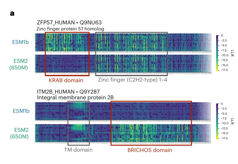
The grey boxes are why this convinced me. A uniformly more sensitive ESM1b would run hotter everywhere; instead the zinc fingers immediately adjacent to KRAB light up in both models. Fig. 1b repeats the comparison as violins over all 519 and all 48 proteins, so it isn’t two cherry-picked genes.

The aggregator. The sign convention trips everyone including me: a score is a log-likelihood ratio of the mutant amino acid against the wild-type one, so lower is more damaging, and the model most confident about a variant is the one returning the minimum. So for each of 20,284 manually reviewed human UniProt sequences, run all eleven models over the wild-type sequence in one forward pass each, then take the element-wise minimum across models of the resulting per-residue matrices. They call it ESMIN: 191.3 million variant scores over 18,683 proteins, precomputed exactly once.

Minimum rather than mean is the decision the paper defends hardest, and correctly, since the obvious objection is that you’ve built a machine for maximizing false positives. Supplementary Note 1 shows minimum aggregation “can substantially outperform averaging when pathogenic LLRs are much more dispersed than the benign” ones, which is the asymmetry ESM actually has. The same note quietly undercuts the method: at fixed class separation, plain averaging eventually wins as you add models. Minimum wins here because eleven is small and the variances are lopsided. The authors proved the shelf life of their own trick, and I respect that they published it.

The distillation. Now train each of the eleven models with a plain MSE loss against ESMIN. Every model is a teacher where it wins and a student where it doesn’t, which is where the “co-” comes from. They unfreeze only the last hidden layer and the LM head, about 3% of the parameters, and because the target is precomputed this decomposes into eleven small independent jobs instead of a distributed ensemble problem. Round one on the 3B model took about 18 hours on one H100; ESM2-35M took 35 minutes. Every model in the family has been downloadable since ESM2 posted in July 2022, so this was never a compute story.

The compression in the title. After round one the models are still complementary enough that averaging pairs beats the singles, which is what the theory predicts: co-distillation raises class separation and evens out the variances, the regime where averaging wins. So rounds two and three take the top four models and average instead of minimizing, with round three moving to 23,803 non-human proteins for fresh signal. ESM2-3B lands on the ensemble line. That is VESM-3B, one model matching an eleven-model ensemble at roughly 61% fewer parameters, then distilled down again into 650M, 150M and 35M backbones that keep >98% of the ClinVar performance. Their schedule ablation is the design fact I’d keep: the first minimum round is what carries it.

We Have Done This Before, With Variant Callers

I couldn’t read this paper without the whole thing feeling secondhand, and it took me a while to place why. This is Genome in a Bottle, rebuilt for language models.

Short-read variant callers disagree with each other in structured, method-specific ways: on indels, on homopolymers, on repeats. GIAB took multiple platforms and callers on the same reference samples, integrated the calls where they could be reconciled, and published the result as truth. Then DeepVariant trained a CNN against that truth set and beat GATK, one of the callers whose output had built the labels. Callers that disagree by failure mode become models that disagree on KRAB versus BRICHOS, GIAB integration becomes ESMIN, and the CNN outperforming its own label sources becomes the student surpassing the teacher.

The genomics version also taught the field what this costs. GIAB’s high-confidence regions deliberately excluded the places the methods couldn’t reconcile: segmental duplications, the MHC, long homopolymers, a pile of clinically important genes. Benchmark numbers marched toward 100% while performance in the hard regions stayed unmeasured, and therefore unimproved, until Wagner et al. curated 273 challenging medically relevant genes back in and it turned out to be visibly worse.

A consensus truth set is only as wide as the union that built it. Co-distillation moves knowledge from the model that has it to the models that don’t. Where no model has it, nothing moves.

The Results That Convinced Me

Every model improves and the small ones are transformed. ESM2-8M goes from 0.66 to 0.88 AUC on a per-gene class-balanced ClinVar set; ESM2-35M goes 0.745 to 0.896, with its DMS Spearman climbing from 0.26 to 0.44. Read that as the small models having had the capacity all along and spending it badly. Extended Data Fig. 3 closes the loop: co-distilled ESM1b now finds BRICHOS and co-distilled ESM2 now finds KRAB. The domains genuinely transfer, which is the strongest evidence against my skeptical reading below.

It tops an independent leaderboard on sequence alone. On ProteinGym’s ClinVar benchmark, roughly 52,000 variants across 2,227 genes, VESM-3B and VESM-650M both land at 0.938 AUC, VESM-150M at 0.936, VESM-35M at 0.929. SaProt, with structure, is 0.921. PoET, with alignments, is 0.920. ESM1b is 0.910. Supervised meta-predictors like REVEL and ClinPred are excluded for circularity, which is the right call: they’re trained on clinical labels, so scoring them on ClinVar measures memorization.

The bar I keep pointing at is VESM-35M at 0.929 against its own base model, ESM2-35M, dead last on the same chart at 0.739. Same architecture, same starting weights, one cheap training step apart. The clinically useful version of that number is the coverage curve: at 90% accuracy VESM-3B can confidently annotate 90% of ClinVar, against 79% for ESM1b, and at 95% accuracy, a level SaProt reaches for only 25% of variants, VESM-3B still covers about 67%.

The allele-frequency control is the best thing in the paper. Take ClinVar, annotate every variant with its gnomAD v4 minor allele frequency, and sweep a threshold that progressively restricts the benchmark to rarer and rarer variants.

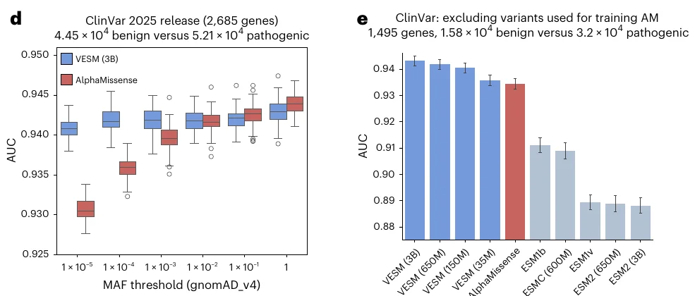
Read honestly, right to left. With no filter at all AlphaMissense is ahead, about 0.944 against 0.943, boxes overlapping, and they stay level down to about 10⁻². Below that AlphaMissense slides to roughly 0.931 while VESM-3B sits flat near 0.941 all the way to 10⁻⁵. Panel e is the cleaner cut: strip out every variant with gnomAD v2 MAF above 10⁻⁵, the data AlphaMissense trained on, and all four VESM models finish above it, though VESM-35M’s margin is a thousandth of an AUC with overlapping error bars.

The interpretation is the authors’ and I think it’s right. Allele frequency really is informative about pathogenicity for common variants, which is exactly why ACMG treats it as evidence. AlphaMissense has that feature and VESM doesn’t, so its advantage is real and inherited from a signal that stops carrying information precisely where the clinical bottleneck is. Ultrarare variants of uncertain significance are the whole job, and there the two swap places. One caveat the paper doesn’t make: VESM is clean of allele-frequency circularity, not of ClinVar circularity in general. ACMG’s PP3 and BP4 codes admit computational predictions as evidence and ESM-family scores are already used that way, so some ClinVar labels have partially absorbed the output of VESM’s own base models.

Then they add structure anyway, backwards. They take ESM3, whose sequence and structure components are cleanly separable, fine-tune only its sequence parameters against VESM-3B’s scores with no structural input, then switch structure back on at inference. That gives VESM3, and averaging it with VESM-3B gives VESM++. Those two are the only models on the chart that take both DMS clusters at once, where alignment-based models otherwise own fitness and activity and structure-based models own binding and stability, and they beat ESM3’s own structure-conditioned scoring on 85% of assays. The claim underneath is that models given structure during training may underuse sequence.

What I’d Push On

The controls here are better than the field norm and I want that on the record before I start. They ran MMseqs2 over training and benchmark sequences together and deleted every training protein that co-clustered with a benchmark one, 5,279 of 18,683. They regenerated ColabFold structures for every structure-based baseline rather than trusting cached predictions. They disclosed that their AlphaMissense filter uses v2 frequencies and therefore leaves 4,818 variants that v4 calls common. None of that is required and most of it goes unrewarded.

Now the parts I’d write in a review.

The leakage control never touched the model they shipped. That MMseqs2 exclusion ran inside the training-size ablation, on ESM2 8M, 35M and 150M. VESM-3B was trained on all 18,683 human proteins, the 5,279 included. So the ablation demonstrates the method generalizes past homology; it does not demonstrate the shipped model is clean of overlap with the benchmark it then tops. The targets are other models’ scores rather than ClinVar labels, so this isn’t label leakage and the benchmarks aren’t invalidated. The main pipeline just gets credited with a sacrifice it never made. Closing it means rerunning all three rounds for the four models that feed VESM-3B: days of one GPU rather than weeks of a cluster. Cheap enough that I’d have made it a condition of acceptance.

The ceiling is the family’s union, and it is never measured. Co-distillation redistributes; it cannot create. Their own ablations point at it: top-8, the default eleven, and all twelve including ESM2-15B land on top of each other, drifting by a couple of thousandths of an AUC in inconsistent directions. That’s saturation, not a scaling law. No experiment in the paper looks for a domain all eleven miss. The benchmarks could show one in principle, since ClinVar labels are clinical assertions and ProteinGym’s are wet-lab measurements, but a ClinVar that pools where clinical attention has already gone means such a domain is more likely under-represented than visible. The clean experiment is to find InterPro or Pfam families where the minimum across all eleven is still uninformative and check whether co-distillation moves them. Predicted answer, no, and it’s a week of analysis on data they already have.

Two hundred proteins should worry us more than they excite us. The headline is that co-distilling ESM2-35M on 1% of the human proteins, about 200 sequences with under 30% identity to anything in the benchmark, reaches 97% of peak ClinVar performance and 94% of peak DMS.

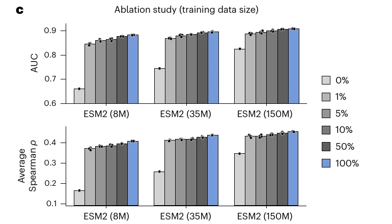
Read the figure as gain rather than as peak and the number changes. ESM2-35M’s ClinVar AUC runs 0.745 untrained, 0.869 at 1%, 0.896 at full data, so 200 proteins deliver about 82% of the improvement; the paper’s 97% is a fraction of final performance, which includes everything the base model could already do. Measuring from AUC’s 0.5 floor instead gives 93%, and that framing is as defensible as mine. Three of them, 97% and 93% and 82%, and the shape is identical in all three: one step, then a long flat run.

It isn’t “just rescaling” — AUC and Spearman are rank metrics, so something genuinely reordered variants. My claim is narrower. Whatever the reordering is, it’s learnable from 200 sequences, which makes it a broad, low-complexity correction rather than memorized per-protein biology. “The collective knowledge of ESM” may be a grand name for a modest recalibration. The counter-evidence is that KRAB and BRICHOS really do transfer between model families, so it’s a live question rather than a settled objection, and the paper never asks it.

“Sequence-only” is doing a lot of work in the abstract. It’s true of VESM-3B. But the state-of-the-art claim in the DMS figure belongs to VESM3 and VESM++, which run ESM3 with structure switched on at inference, and which the authors’ own License section flags as derived from a model “available under a noncommercial license agreement.” Two headlines, one adjective between them. The sentence a team should take away: the best deployable model is VESM-650M, tied with the 3B at 0.938, and that’s a licensing answer rather than a performance one. And when your top three tie to three decimals you’re measuring the noise floor of the instrument, not the models.

One last thing, from the back matter: Nature Methods names Milot Mirdita as a referee, and the acknowledgements credit him with the suggestions “leading to the iterative co-distillation approach presented in this work.” Rounds two and three, the compression in the title, came out of peer review. I’ve spent a fair amount of this series being impatient with how slow publishing is. This is the counterexample.

The Data-Infrastructure Coda

I do data infrastructure for a living; TileDB-SOMA is my day job, so treat everything below as an interested party’s reading. The methods section lands differently on me than the results do. This paper’s compute problem is solved and its distribution problem is not.

The compute was eighteen hours on one GPU. The artifact is bigger: 216 million precomputed missense scores covering all 20,421 human UniProt sequences, plus 71 million coding SNPs on hg38 and hg19, for several separate models, distributed as files. One dataset has to serve two irreconcilable access patterns. A clinical pipeline arrives holding a VCF and wants scores by (chr, pos, ref, alt): sparse, scattered, joined against a variant list. A protein scientist arrives holding a UniProt accession and wants the entire 20 × L slab: dense and contiguous. The authors solved it by shipping both as separate downloads, and that duplication is the tell. Then there’s the axis nobody planned for: ESMIN is a reduction, and the ablations recompute it over the top three, the top eight and all twelve, so which models went into a score is a query rather than a filename.

Which brings me to the part I actually care about, the same one I landed on reading about cell-type labels two weeks ago. A model score is an opinion with a version number. The rule is already written down: ACMG’s sequencing standards have required since 2013 that a clinical lab “capture the specific version of each component of the pipeline utilized in the analysis of each patient test.” What’s missing is the join. This single publication produces seven score sets, round four is explicitly on the table, and a lab that returned an interpretation using VESM-3B has to reproduce it after the weights move. “Which model produced this call” should be answerable from the call, not from somebody’s lab notebook. That isn’t a modeling problem, and it’s the half that outlives the model.

The thing I keep coming back to isn’t the leaderboard. It’s that this was free, and it sat there. Eleven models had already found the KRAB domain and the BRICHOS domain and everything else in the union. The weights were on the internet, the compute was one GPU, and the whole contribution is asking all eleven at once and then asking again. I don’t fully believe the framing that this recovers “the collective knowledge of ESM.” I do believe the finding underneath it: that pooling these models helped was already on the leaderboard, but what the leaderboard never showed is which residues each one was getting wrong, and that answer turned out to be specific enough to act on.

Which leaves the question the paper can’t answer with the benchmarks it has: what sits in the intersection of all eleven blind spots? There’s a domain family somewhere that every ESM model calls neutral and that matters to somebody’s kid. Co-distillation won’t find it, because co-distillation only moves what some model already has, and ClinVar’s evidence pools where the clinical attention already is, which is precisely not where an unexamined domain lives. GIAB needed a separate, deliberate, years-long curation effort to find its own hard regions. Somebody is going to have to do that here too, and it won’t look like a better model.