Journal Safari: Seven Million Parameters and a MacBook Air

The first paper in this series was a 500-million-parameter foundation model trained on 68 million cells. I spent most of that post poking holes in its interpretability trick, but I never questioned the premise: that the way forward in single-cell was more cells and more parameters.

Then I read a preprint that argues the opposite, by being smaller and winning anyway.

Pan-human Azimuth (Sarkar, Li et al., bioRxiv, posted 21 July 2026) is a 7-million-parameter classifier. It runs on a MacBook Air. It annotates cells about seventy times more cheaply than the model I read in July, and on the one task both can do, it wins. The authors are explicit that the model is not the contribution. The contribution is the labels.

Standard disclaimer, and a real one this time: this is a preprint. Not peer reviewed, posted two weeks ago, and licensed CC BY-NC rather than the CC BY of the last two papers I covered. Installment #1 had Nature Communications’ transparent referee reports to check my reading against, which was a genuinely humbling exercise. Here there’s nothing. So this post is me being the referee, with all the overconfidence that implies.

Why This Paper

Single-cell is drifting toward reference-based annotation, not agreeing on it. Nobody agrees on the reference, and there are two ways to be wrong about it.

The first is one reference per organ, which is what Azimuth itself has been since the pandemic, along with DISCO and CellTypist. Each tissue gets its own curated model and its own naming committee. This works fine right up until you want to compare across tissues, at which point you discover you can’t: if your lung reference says “fibroblast” and your heart reference says “SCN7A+ fibroblast,” the question “are heart and lung fibroblasts different?” has been pre-answered by two groups of people who never talked to each other.

The second is foundation models. scGPT, SCimilarity, and friends build a self-supervised embedding from aggregated public data, then read labels off it: SCimilarity by nearest-neighbor lookup, scGPT by fine-tuning a classifier. Either way you inherit what the reference’s original authors called things. The paper has a name for the failure mode: label fragmentation. The paper’s exhibit A is beautiful. One population in CELLxGENE goes by “respiratory goblet cell,” “mucus secreting cell,” “mucus secreting goblet cell,” “secretory cell,” and “native cell.” Five names, one cell type, garbage vocabulary in and garbage vocabulary out.

Pan-human Azimuth’s answer is to stop arguing and commit: one tree for the entire human body, one classifier trained on all of it, and a calibrated confidence at every level so the model can tell you when it doesn’t know.

What They Actually Did

The coffee-length version: they collected 27 million cells and then spent the paper’s real effort throwing most of them away.

The corpus. 27.04 million cells across 23 tissues, from five repositories: 123 datasets from CELLxGENE, 215 from HuBMAP, plus DISCO, Azimuth, and GTEx references. Because the same GEO submission shows up in three of those hosts with different processing, they built a near-duplicate detector: random Gaussian projection to 100 dimensions, then flag anything landing within a Euclidean distance of 1 of a reference cell. Cheap, clever, and a tell about what kind of project this really is.

Then three curation passes, each a small piece of machine learning doing librarian work. Harmonize: Seurat’s anchor-based label transfer relabels every cell into one shared vocabulary. Error-correct: cluster each dataset at high resolution, and where a cell disagrees with its cluster’s majority, let a ridge logistic regression on up to 100 markers per side break the tie. About 7% of cells got reassigned. On a 27-million-cell corpus that’s roughly 1.9 million cells whose first automated label was simply wrong. QC-filter: a one-vs-all marker model scores every cell against its label, keep anything above 0.75, then cap each cell type at 25,000 cells per tissue so B cells don’t drown out pulmonary ionocytes.

27.04 million cells in. 9,665,434 out.

The tree. They didn’t invent a taxonomy, which was the right call. They adopted DISCO’s, itself derived from expression data rather than anatomy textbooks, patched it, and then did the deeply unglamorous work of mapping every node and leaf 1:1 to a term in the Cell Ontology. Eight levels, running 13 → 91 → 209 → 313 → 355 → 374 → 380 → 382 classes. That crosswalk is the difference between “here is my private naming scheme” and “here is a translation into the vocabulary everyone else already uses,” and there are professional ontologists on the author list because somebody had to do it.

Two design decisions carry the whole thing, and both are about knowing when to stop. First, the tree has ragged edges and the model is allowed to quit early: a GZMK+IL7R+ CD8 T cell is eight levels deep because immunologists have subdivided T cells to death, while a club cell bottoms out at three. Shallow paths are padded with blanks, and each head can output “blank,” meaning this is definitely a T cell and I decline to guess which kind. Second, a non-cell class. Instead of bolting QC on beforehand with UMI cutoffs, they trained on negative examples: real empty droplets from 20 public 10x demo datasets, plus 5,000 simulated profiles per tissue for the high-UMI clumps a cutoff would never catch. About 145,000 negatives labeled “Unassigned,” so the classifier does quality control and annotation in one pass with no arbitrary threshold.

The model itself is almost anticlimactic: 5,055 genes squashed to a 128-dimensional embedding, then eight small MLP heads hanging off it, each seeing the embedding plus a compressed version of every shallower head’s output. 6,981,993 parameters, 38 epochs, one A100. Per-head temperature scaling brings expected calibration error to 0.0044, which matters enormously, because the whole downstream workflow is “filter at confidence ≥ 0.75” and that threshold is meaningless if the numbers are lying to you. Inference runs at roughly 1,000 cells per second on an M2 MacBook Air, no GPU required.

We Have Done This Before, With 16S

I have to say this out loud, because it reframes what kind of paper this is. Pan-human Azimuth is a taxonomic classifier. Not metaphorically, structurally. The RDP Classifier scores a 16S read against every genus in a fixed taxonomy running domain to genus, bootstraps that call a hundred times, then sums the support upward through the ranks and reports the deepest one still clearing 80%; below that it stops and says “unclassified Bacteroidetes.” Swap read for cell, rank for level, and bootstrap support for calibrated confidence, and the behavior is identical, abstention included. The computation is inverted, though: RDP assembles its hierarchy from the bottom, while this paper’s eight heads are each conditioned on every shallower one. Kraken 2’s lowest-common-ancestor assignment is a version of the same reflex.

Which matters because the field’s central bet here has already been tested elsewhere, over about fifteen years, and 16S’s verdict was that the taxonomy is the hard part. Not the only part, but the part that outlives the software. That is precisely the argument for 7 million parameters over 9.65 million harmonized cells instead of 500 million over 68 million author-labeled ones.

But 16S also taught the cost. When GTDB redrew bacterial taxonomy on genome evidence, 58% of the 94,759 genomes in it changed classification, and a decade of Greengenes-labeled results needed re-reading. A shared vocabulary makes studies comparable and simultaneously freezes one naming decision into every downstream result. The Cell Ontology crosswalk is the right mitigation. Versioning the taxonomy is now a first-class problem. GTDB numbers its releases; nobody has solved the re-reading.

That parallel runs deeper than one section can hold — particularly what 16S learned about contamination, and what it should be telling single-cell right now. That’s the next post.

The Results That Convinced Me

Three, in descending order of how much I believe them.

It generalizes to unseen donors. They ran the whole 1.1-million-cell, 28-tissue Tabula Sapiens atlas in one inference pass, including nine donors released after the model was trained, with no confidence drop for the new ones. Immune and stromal labels come back finer than the human annotations, because T-cell structure learned in immune-rich tissues transfers into lung.

It found a cell type where it had never seen one. It called hematopoietic stem cells in spleen — a population entirely absent from the corpus — from patterns learned in blood and bone marrow. The markers check out and the biology backs it up: the human spleen is a documented reservoir of hematopoietic stem and progenitor cells, quiet at steady state but ramping up during stress erythropoiesis. The cells really are there to find, and knowledge crossed tissues because the hierarchy let it. That’s the single best argument for organism-wide training over per-organ references.

It overruled the humans, correctly. Only 0.3% of Tabula Sapiens came back “Unassigned,” good in itself for a hand-curated atlas. But the largest bucket of disagreement was cells the curators had labeled neutrophils, and those cells lack FCGR3B and show no coherent myeloid signature at all, while cells both methods call neutrophils express it fine. Neutrophils are a miserable case for droplet scRNA-seq: low RNA content, fragile, easily swamped by ambient signal. The empty-droplet training caught human error.

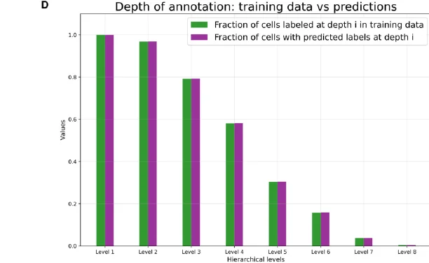
Figure 2 is where the paper is most honest about itself. Its accuracy panel shows non-blank labels decaying from about 1.00 at level 1 to roughly 0.83 at level 8, and 83% across 382 classes is genuinely strong. But look at the panel above: 97% get a level-2 label, 58% reach level 4, and essentially none reach level 8. Eight levels of resolution is real and very thin at the bottom. Most cells land at level 3 or 4, which is a perfectly useful place to land. It’s just not the number in the abstract.

Then the scale run, where the cheapness of the model stops being a curiosity and becomes the point. They annotated scBaseCount, still scBaseCamp in the preprint, 85.9 million non-cancer human cells machine-scraped from public archives and completely unannotated, in 13.5 hours on one A100. And the “Unassigned” class earned its keep: 0.3% on hand-curated Tabula Sapiens, 11% on scBaseCamp, where the flagged profiles have a median UMI count of 19 against 4,734 for everything else. That’s not a subtle judgment call, that’s obvious garbage, caught with zero threshold tuning.

The refusal reflex shows up best in the spatial section. Run the model on Visium HD kidney at the 8 µm bins everyone uses and each bin straddles multiple cells, so the profiles are mixtures that violate everything the model was trained on. 69% came back “Unassigned.” It correctly refused. Switch to bins that follow inferred cell boundaries and assignment jumps to about 80%. A model without an abstention class would have returned 100% confident garbage and nobody would have noticed.

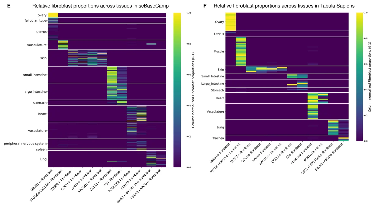
The biology payoff is the fibroblasts, and it could only exist because of the shared vocabulary. How much fibroblasts specialize to the tissue they live in is a live question, not settled knowledge: the most relevant prior is a 2021 cross-tissue atlas that integrated roughly 230,000 fibroblasts across 17 tissues and found two universal subtypes seeding specialized ones downstream, largely in mouse. Asking it in human was blocked by something mundane, in that every organ atlas named its own fibroblast subtypes independently. Apply one hierarchy across ten thousand datasets and the answer is a continuum. G0S2+ PPP1R14A+ fibroblasts show up in over 60% of lung samples and in under 0.1% of non-lung samples, where the handful of apparent exceptions got chased down and turned out to be mislabeled lung: two accessions filed under “musculature” in scBaseCamp are recorded as lung in ENA. The model was more right than the metadata.

What I’d Push On

Now the part where I earn the word “safari.”

The ground truth is model output. There is no fresh human annotation anywhere in this pipeline. Every training label came from transfer off an existing reference, was adjudicated by regressions trained on that same reference’s markers, then filtered by more of the same. To be fair, nobody can hand-annotate 27 million cells and their three-pass pipeline is thoughtful about catching its own errors. But be clear-eyed about what the model therefore is: a fast, calibrated, hierarchically aware compression of what Azimuth, DISCO, CellTypist and the Human Brain Cell Atlas already believed. It cannot discover a cell type those references got wrong, and when it disagrees with them that disagreement is noise reduction by construction, not new knowledge. The splenic HSC result is the closest thing to an exception, which is why it matters more to me than any benchmark number.

The benchmark rewards coherence, not truth. Because no two tools share a vocabulary, they invented a differential-expression-based diagnostic they call “DE separability”: take a method’s labels, derive the top 10 differentially expressed genes per label, train a logistic regression on only those genes, report the accuracy. It’s a thoughtful way around an impossible comparison problem, and the failures it surfaces are real — SCimilarity put lung epithelial cells in cardiac muscle with no cardiomyocyte markers anywhere, which is not a naming disagreement.

But look at what the metric measures. You derive markers from the labels, ask a linear model to recover the labels from those markers, and report in-sample training accuracy with no held-out split. A self-consistent labeling scheme scores high by construction, and Pan-human Azimuth’s labels came from a pipeline that explicitly deleted internally inconsistent cells, so it was optimized for the property being measured. Worse, collapsing two distinct cell types into one label raises the score and splitting finely lowers it, so the metric penalizes exactly the resolution the paper sells as its advantage. Their own supplement half-admits it: manual stomach annotations score highest of all, while annotating at lower resolution. The baselines also ran at tutorial defaults, SCimilarity in unconstrained mode, when that same tutorial documents a constrained mode that would likely have prevented the cardiac-muscle call. I don’t read that as gamesmanship; it’s the well-documented optimistic bias that shows up whenever a method’s authors also configure its competitors. But the gap is softer than the figures make it look.

Most headline numbers are measured after filtering. The downstream panels in Figure 3 drop cells that fail hierarchical consistency or fall below 0.75 confidence. That’s correct practice and they document it every time. But “median confidence 0.89” on scBaseCamp describes the ~75 million survivors of the model’s own gates, not the 85.9 million it started with.

Scale is hitting diminishing returns, and they said so. Their own supplement shows accuracy gains going gradual past roughly 5 million training cells. Credit for publishing that, since it cuts against the easiest way to write a follow-up paper. It also means the ceiling is set by label quality rather than data volume, the strongest possible version of their own thesis. More cells from well-represented tissues will not help. The missing coverage is development, disease, cancer, and the tissues outside the 23.

And the input layer will be a problem in spatial. The model eats a fixed 5,055-gene vector. Visium HD could feed it, being sequencing-based and genome-wide, but most imaging platforms read targeted panels, and panel size turns out to be the wrong thing to measure. What matters is which genes. CosMx’s whole-transcriptome imaging, which reads 19K RNAs alongside protein off the same FFPE section, is plausibly in business. Xenium’s 5,000-gene panel is not, despite the matching headline number: only 1,784 of its 5,001 targets appear in the model’s published feature list. The misses include PTPRC, LYZ, ACTB and B2M, much of the high-expressing core a log-normalized profile leans on, and also G0S2 and PPP1R14A, the two genes this paper’s own fibroblast result rests on. Lower still is G4X from Singular Genomics, my old shop, at 500-plex, trading transcriptome breadth for RNA, protein, and H&E off one FFPE section. And nothing stops you running any of them: the shipped package zero-fills whatever’s missing and returns a calibrated confidence anyway. The paper never raises it, and it’s the gap I’d expect to bite first.

The Data-Infrastructure Coda

I do data infrastructure for a living, so here’s what jumped out reading the methods: the scientific contribution is a set of labels, the engineering contribution is a corpus, and the corpus was harder. Five hosts, near-duplicate detection, then layer after layer of per-cell metadata: transferred label, cluster-majority label, classifier verdict, QC score, eight hierarchical labels, eight confidences, a consistency flag. Every one is a column of annotation. The counts barely change; the annotations are the entire story.

That’s a sparse-array-plus-metadata problem, and I don’t have to argue it by analogy, because one of their five sources already is one: the CZ CELLxGENE Census is built on TileDB-SOMA, which is my day job, and they pulled 123 of their ~370 datasets through its API. Their balanced subsample — everything above 0.75, capped at 25,000 per type — is a metadata query over 27 million cells that then slices the counts. That’s the query pattern this storage shape exists for.

The part I keep chewing on is versioning, because annotation is an opinion with a version number, and almost nobody keeps two of them. Nothing stops you: their own benchmark carried four competing label sets on one dataset, and the Census pins dated releases, which is how this paper read one. It’s convention, not capability. Re-annotating overwrites the column you had, so where do v1 and v2 disagree on these cells is a question nobody thinks to ask. For regulated work that’s worse than inconvenient: if a filing rests on an analysis you need to reconstruct that exact labeling later, and reproducing terabytes is a bad way to do it when pinning a version would do. None of which is a complaint about the authors, who shipped fine with h5ad files. The claim is only that the next version of this corpus will hurt more than this one did.

The through-line across three installments is starting to embarrass me a little. A 500-million-parameter foundation model, half a million whole genomes, and now a 7-million-parameter classifier over 23 tissues, and in all three the thing that will still be useful in five years is the data artifact: the structural-variant catalogue, the harmonized corpus, the Cell Ontology crosswalk and marker tables already merged into HuBMAP’s reference tables. The modeling dates fastest. Which is a strange thing to conclude from a paper whose headline is a model, except that it’s the paper’s own argument, and it’s why I think this one is right even where its benchmark is weak. Curate the labels, keep the tree small enough that a human can argue with it, then let the model decline to guess.

Next time I want to stay with that 16S parallel, because there’s a part of it the field should be more nervous about than it is.