Journal Safari: What Do You Buy by Sequencing Half a Million Whole Genomes?

Two weeks ago I kicked this series off with a 500-million-parameter single-cell model and spent the whole post poking at its interpretability trick. This time there’s no trick to poke at, because there’s no model. The paper is a resource: the UK Biobank Whole-Genome Sequencing Consortium finished sequencing the genomes of every last one of its 490,640 participants (Nature, 2025, open access), and the deliverable is the dataset itself.

That changes the job of a close read. When the output is a dataset and not a method, “is it correct” is the wrong question — nobody’s arguing the sequencing is wrong. The right question is the one a grant reviewer would ask: was it worth it? We already had these people genotyped on an array, and we already had their exomes. What does sequencing the whole genome, deeply, buy on top of that — and what does it cost after the machines stop running?

Why This Paper

The UK Biobank has been genotyped three times over, each rung of the ladder seeing deeper into the genome. First a SNP array plus imputation (2018), good for common variants and cheap, blind to rare ones. Then whole-exome sequencing (2021), which nails the protein-coding 2–3% of the genome and misses everything else. Now whole-genome sequencing: every position, at a mean of 32.5× coverage, for all 490,640 people. The direct predecessor was a 150,119-genome release in 2022; this is the completion of that program at more than triple the size.

The scientific case for the top rung rests entirely on one premise: that rare, non-coding variation matters — that disease-relevant signal is hiding in the 97% of the genome that isn’t protein-coding, and that it’s rare enough that arrays and imputation can’t reach it. The field mostly believes this. Whether this paper cashes it out is the whole game, and it’s why I read past the abstract’s big multiplier and went looking for which specific results actually needed WGS to exist.

What They Actually Did

The coffee-length version: sequence everyone deeply, then call the variants several different ways because the project ran for years and the tools kept improving.

Sequencing was done on an Illumina NovaSeq 6000 at 32.5× mean coverage, with 1,175 samples run in duplicate for QC and Genome in a Bottle reference materials for accuracy checks. For SNPs and indels they produced three call sets: a GraphTyper joint-calling set (~1.04 billion SNPs, 101 million indels) plus single-sample and aggregated sets from Illumina’s DRAGEN caller. Structural variants came from DRAGEN-SV combined with a long-read study and seven assemblies, then re-genotyped with GraphTyper for consistency: 2.74 million SVs. Ancestry cohorts were defined against gnomAD — 458,855 non-Finnish European, then 9,674 South Asian, 9,229 African, 2,869 Ashkenazi Jewish, and 2,245 East Asian.

Two things to file away. Hold that ancestry breakdown — 458,855 of 490,640 are one group. And the three-call-set situation is real friction: GraphTyper and the two DRAGEN sets don’t agree perfectly, and if you’re a downstream researcher, you have to pick one. Not a flaw exactly — the authors frame it as “a diversity of approaches” reflecting the project’s timeline — but it’s a choice they’ve pushed onto every user of the resource.

The Genuinely WGS-Only Wins

If you want the cleanest “you needed whole-genome sequencing for this,” it’s structural variants. Arrays and exomes are essentially blind to them, and this call set has 2.74 million — about 13,102 reliably called per person, versus 7,439 per person in gnomAD-SV. And they’re overwhelmingly rare: 76.3% are carried by fewer than 10 individuals. The rare deletions run long (median 1,660 bp) while common ones stay short (169 bp), which is exactly what selection predicts — big deletions are deleterious, so they get kept rare. The stat that made me sit up: by base pairs affected per genome, SVs (3.6 Mb) move more sequence than SNPs (2.9 Mb) and indels (1.5 Mb) combined.

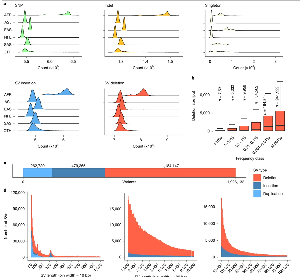
Here’s where my microbiology past kicked in. The consortium downsampled from 1,000 up to 490,541 genomes and watched variant discovery accrue, and the curve behaves exactly like a rarefaction curve in ecology. Common variants (>1% frequency) saturate almost immediately — there are only so many positions polymorphic at that frequency in humans, so a few thousand genomes exhaust them. But the rarest class (≤0.001%) is still climbing at 490,000 genomes with no plateau in sight. That’s the human version of the rare biosphere: the 16S survey saturates the dominant taxa fast, and shotgun metagenomics keeps turning up the long tail no matter how deep you go. If the rare-variant curve never flattens, no biobank is ever “done” — which is precisely why the cohort keeps growing (150k → 490k → 500k+).

The other clean win is human knockouts. Half a million genomes give you 10,071 autosomal genes with at least 100 heterozygous loss-of-function carriers, and 1,202 genes with three or more homozygous carriers — natural experiments in switching a gene off, the human equivalent of a knockout mouse and the closest thing you get to a preview of what inhibiting that target with a drug would do. On the clinically actionable side, across the 81 ACMG secondary-findings genes they found 7,313 pathogenic or likely-pathogenic variants in 51,107 people, with SVs bumping the count of individuals with an actionable genotype by nearly 15%.

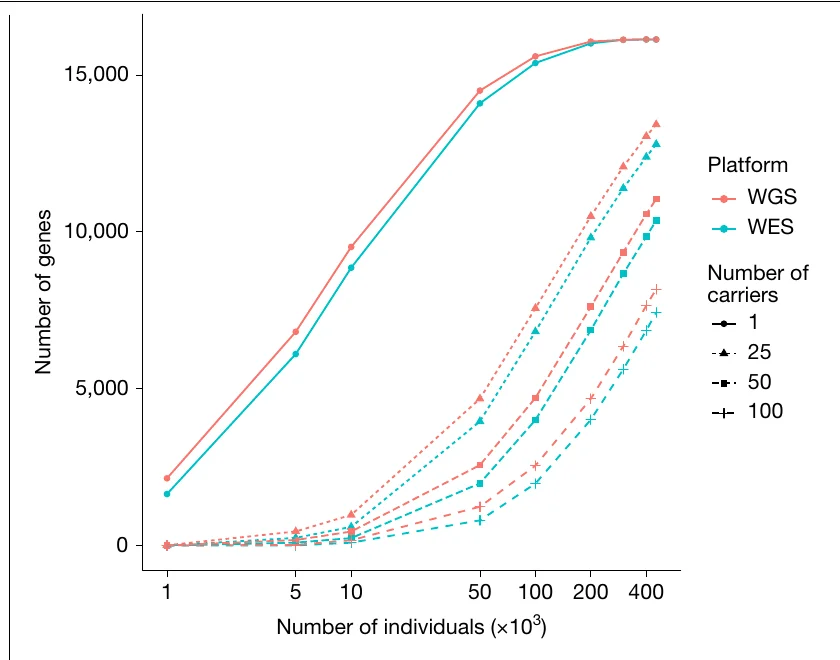
That figure is also where the honesty starts. WGS beats WES on knockout discovery because it covers coding regions more evenly, not because it sees different biology — and the margin is modest.

Where WGS Only Ties WES

This is the result I’d make everyone stare at. The consortium ran the same rare-variant collapsing PheWAS on the same 460,552 people, once on the WES coding regions and once on the WGS coding regions. Result: 1,359 significant gene–phenotype associations, of which 1,188 were significant in both technologies. WGS found 105 (7.7%) that WES missed; WES found 66 (4.9%) that WGS missed. The Spearman correlation of the p-values was 0.95.

For protein-coding genes, in other words, whole-genome sequencing is a marginal upgrade over the exome you already have. Its coding advantage is purely coverage evenness — no exome-capture dropout — which rescues awkward regions like the MHC (WGS-unique hits in HLA-C and C2) and cuts the number of genes with poor coding coverage from 1,299 in WES to 638 in WGS. Real, but incremental. Which means the entire justification for the extra spend has to come from what the exome can’t see at all.

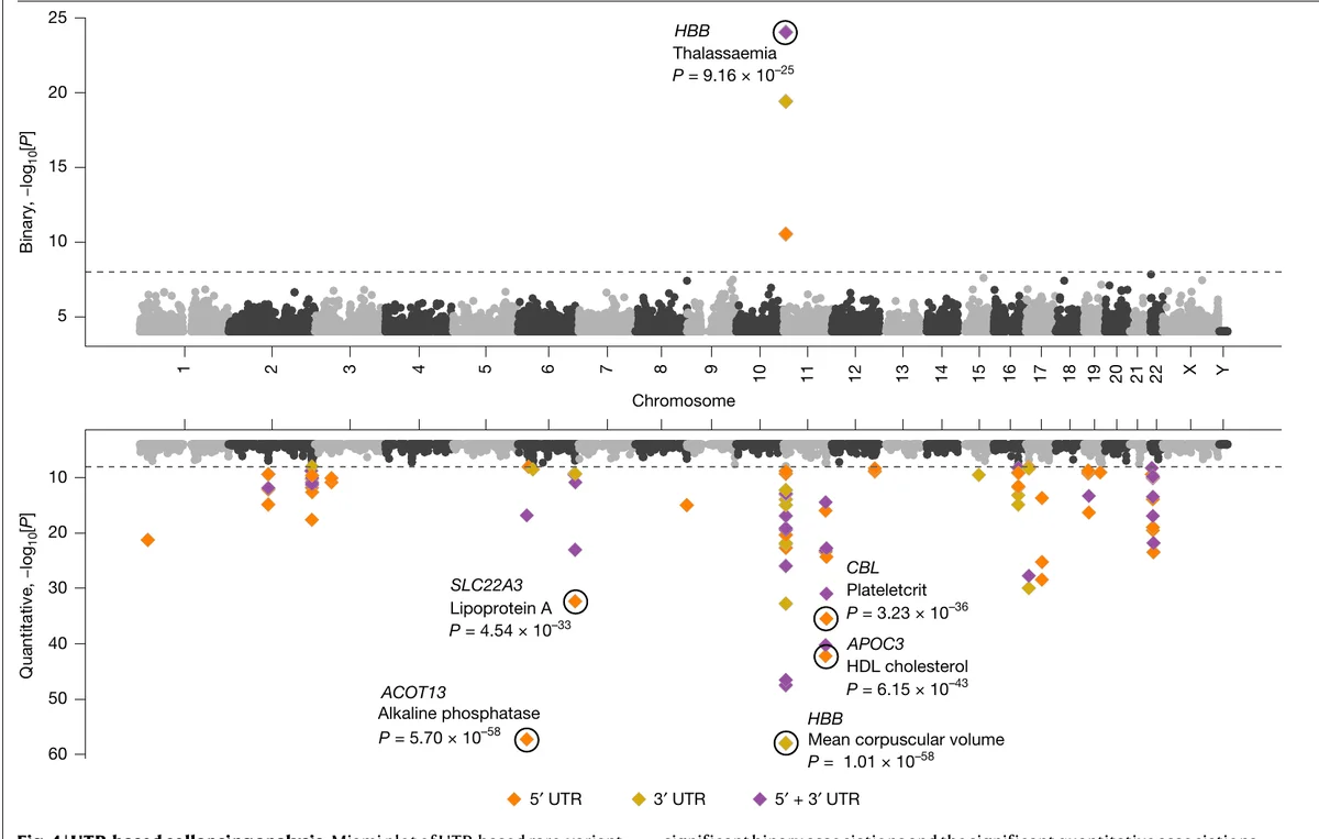
So the load-bearing result isn’t a nice-to-have — it’s the non-coding one, and everything rides on it. Whole-exome capture misses roughly 69% of 5′UTR and 89% of 3′UTR variants, so a rare-UTR analysis is only possible with WGS. The consortium collapsed 13.4 million rare (MAF < 0.1%) UTR variants per gene and tested them, getting 63 significant associations across 32 genes — and it recovered textbook signal from UTRs alone: HBB and thalassaemia, APOC3 and HDL, SLC22A3 and lipoprotein(a), CBL and plateletcrit.

What I’d Push On

The “global health” framing is a bit misleading. The cohort is 93.5% non-Finnish European. The other cohorts — 2,245 to 9,674 people each — are genuinely valuable (the South Asian cohort is roughly four times the size of gnomAD’s South-Asian genomes), and they buy real biology a European-only study can’t: the trans-ancestry meta-GWAS turned up 82 signals significant only outside the European group, and the malaria-selection story is beautiful, with the G6PD deficiency variant at 14.7% frequency in the African cohort versus 0.005% in the European one. But 9,000 people against 458,855 is a rounding error, and an abstract that ends on “improve global health” is describing an aspiration, not this dataset. The honest version came up in my own reading over and over: if you actually cared about the diversity dividend, you’d sequence the populations where human genetic variation is deepest — Africa — at scale, and nobody is funding that at half-a-million-genome depth.

Most of it is re-confirmation, not discovery. The marquee genes — HBB, G6PD, APOC3 — are all textbook. The paper’s own novel fraction is 16.6%. That’s completely fine for a resource paper; the point of a resource is the resource, not new biology. But it should be filed as a resource paper, not read as a discovery one.

The non-coding causality is unproven by the paper’s own numbers. Of the significant UTR hits, 83% have a common variant within 500 kb tagging the same trait, and 51% overlap a coding signal. So how many are independent causal UTR effects versus LD shadows of things we’d already find through the array or exome? The honest core is the 10 associations that show up only when UTRs are added to the coding model — that’s the clean evidence non-coding variation adds something, and it’s a much smaller number than 63.

Unlike last time, there’s no transparent peer-review file to check my objections against. Nature Communications publishes its referee reports by default; the flagship Nature only does when authors opt in, and these authors didn’t — the page names one reviewer (Yukinori Okada) and some anonymous others, but no reports. So this critique is my own read plus the paper’s own admissions, which to their credit are right there in the text if you read past the abstract.

The Data-Infrastructure Coda

I do data infrastructure for a living, so the number that actually keeps me up isn’t 1.5 billion variants — it’s where they live.

Start with the sequencing economics, because they’ve quietly inverted. A 30× genome is now roughly $100 at scale on the newest platforms, essentially at parity with a whole exome and only about twice the cost of an array — for far more content. On a variants-per-dollar basis WGS already won, and that’s why every big biobank switched. But “variants per dollar” is a vanity metric: most of that content is rare, non-coding, unknown-effect, and the coding portion only ties WES. The cost didn’t disappear when sequencing got cheap. It moved downstream.

Here’s the downstream. 490,640 people at ~25 GB per CRAM is about 12 petabytes of reads. Let those go cold in Glacier Deep Archive and it’s ~$150k/year — but cold means hours-to-restore and retrieval fees, so it’s not queryable in place. Keep it hot in S3 Standard so researchers can actually use it and you’re looking at ~$3.4M/year, every year. And egress is the quiet killer at ~$0.09/GB — moving a single petabyte out costs ~$90k, which is exactly why the UK Biobank forbids download and makes you compute inside its Research Analysis Platform. The value of a biobank is being queried and re-analyzed by thousands of researchers, and that — hot storage plus compute plus egress — is the recurring bill, not the one-time sequencing.

Which is a specific data-shape problem. 490,640 samples × ~1.5 billion variants is a giant, extremely sparse sample-by-variant matrix, and the joint-called pVCF the field defaults to blows up combinatorially — asking “who carries variant X in ACMG gene Y” means scanning enormous files, and every time the cohort grows you re-generate the whole thing. That maps almost too cleanly onto storing variants as cloud-native sparse arrays. TileDB-VCF models population variant data as 3D sparse arrays where sparsity is a feature you exploit rather than a tax you pay: you slice by genomic region × sample × annotation without materializing the full matrix, and you ingest new genomes incrementally instead of re-joint-calling everyone — which is the exact growth pattern (150k → 490k → 500k+) a biobank has. The consortium already proved out the underlying principle, incidentally: the Sanger-sequenced portion was processed on a commercial cloud-genomics platform (Velsera Seven Bridges), co-locating compute with storage specifically to “minimize data transfer steps.” Moving compute to the data is settled; exposing it as a genuinely queryable variant store — rather than running batch workflows over files — is the complementary step, and TileDB-VCF’s sparse arrays already do exactly that.

The thing I keep coming back to: making the genome is solved. Sequencing fell off a cost cliff, and the paper is the proof — you can now afford to do the whole cohort, deeply, and find the rare tail you couldn’t see before. But the rare tail never saturates, the cohort never stops growing, and the resource is only worth anything if half a million genomes stay queryable and re-analyzable for the next decade. WGS didn’t eliminate the hard problem. It relocated it, from the sequencer to the storage engine. That’s a trade I’ll happily take — but it’s worth being clear-eyed that we made it.

See you in two weeks with the next one.